Deprecated: Creation of dynamic property Pusher\Log\Logger::$file is deprecated in /html/wordpress/wp-content/plugins/wppusher/Pusher/Log/Logger.php on line 18
Deprecated: Creation of dynamic property Pusher\Log\Logger::$file is deprecated in /html/wordpress/wp-content/plugins/wppusher/Pusher/Log/Logger.php on line 18
Deprecated: Creation of dynamic property Pusher\Dashboard::$pusher is deprecated in /html/wordpress/wp-content/plugins/wppusher/Pusher/Dashboard.php on line 68
Deprecated: Creation of dynamic property Pusher\Log\Logger::$file is deprecated in /html/wordpress/wp-content/plugins/wppusher/Pusher/Log/Logger.php on line 18
Deprecated: Creation of dynamic property Pusher\Log\Logger::$file is deprecated in /html/wordpress/wp-content/plugins/wppusher/Pusher/Log/Logger.php on line 18 abap Archives - j&s-soft
The following exercises will help you understand some basic concepts in ABAP.
“Tell me and I forget, teach me and I may remember, involve me and I learn.”
Benjamin Franklin
On exercism.org you will find 40 ABAP exercises. These are common programming exercises such as Word Count, Tic-Tac-Toe, Scrabble Score and so on that you will probably come across in one way or another when learning a programming language. We recommend that you register there and start doing all these exercises to build up your knowledge of programming and ABAP.
What our blog series Introduction to ABAP will do for you:
Discuss the task and the considerations you need to make to solve the exercise without having to look up a published solution.
Randomly show you some ABAP peculiarities that come up in each exercise, so that you understand ABAP better and better.
Work out the prime factors of a given natural number.
A prime number is only evenly divisible by itself and 1.
Note that 1 is not a prime number. Some more useful school knowledge: Factors are the numbers you multiply together to get another number. For example: Factor 2 * Factor 3 = 6. “Prime factorisation” is working out which prime numbers can be multiplied together to make the original number.
2. An example to help you understand in depth.
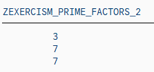
What are the prime factors of 147?
It’s best to start with the smallest prime, which is 2, so let’s see:
Can we divide 147 exactly by 2? 147 ÷ 2 = 73½ No, you can’t. The answer should be an integer, and 73½ is not an integer.
Let’s try the next prime number, 3: 147 ÷ 3 = 49 That worked, now we try to factor 49.
The next prime number, 5, does not work. But 7 does, so we get 49 ÷ 7 = 7.
This is as far as we need to go, because all the factors are prime numbers. 147 = 3 × 7 × 7
Now you have a better understanding of this problem. Have you?
3. What are the constraints of the task?
There is no need to scroll up to see the task again. Here it is:
Calculate the prime factors of a given natural number. A prime number is only evenly divisible by itself and 1. Note that 1 is not a prime.
line of code
constraint
coding
1
an input (natural number) is given.
input (natural number)
2
there will be an output of prime factor(s)
output
3
The smallest prime is 2, that is why we will start prime factorization with divisor 2.
divisor = 2
4
How do you get only evenly divisible numbers? Answer: by using the modulo operation (“MOD” or “%” in many programming languages). The modulo operation is the remainder of the division.
For example, 5 mod 3 = 2, which means that 2 is the remainder when you divide 5 by 3. If there is a remainder, the number hasn’t been divided equally. For our problem, we would need 5 mod 5 = 0. No remainder, so evenly divisible.
More generally: Input MOD divisor < > 0, tells us that the input is not evenly divisible by this divisor and therefore we can’t proceed, we need to change the divisor.
if input MOD divisor < > 0
5
We try the next possible divisor, so add 1 to it and try again.
do divisor + 1, start again at line 3
6
If input MOD divisor = 0, store divisor as prime factor in our output or in other words: if line 3 of the code is not true (else) store divisor as prime factor in our output
else write divisor as prime factor in our output
7
Since we have found a prime factor, we can proceed, so we actually divide the given input by the divisor: input = input DIV divisor, starting again with the “new” input at line 3.
input DIV divisor start again at line 3
8
When do we need to stop this loop?
As you can see, our first input (line 1) is getting smaller and smaller. It has to stop when there is no prime factor left. That is, when the input is equal to 1.
Stop this calculation block when the input is 1. Right? If you reverse this constraint: Run as long as input is greater 1.
start again until input > 1
Once you understand this, it is actually quite simple. 8 lines of code.
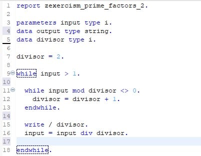
Okay, you’re right, we’re not done yet. Actually, we need 12 lines of code to translate our reflections into ABAP. As you can see here:
4. Our solution translated in ABAP.
Note: On exercism.org you will find solutions using classes and methods to calculate prime factors. As our blog series is aimed at complete programming beginners, we skipped the object-oriented programming (for now) and wrote a simple ABAP report.
5. Basic ABAP knowledge you need to know to understand the ABAP code above.
ABAP Syntax
Typically, an ABAP statement starts with a keyword and ends with a period. For example:
Unlike other languages such as Java or C#, ABAP is not case-sensitive. This means that you can use the ABAP keywords and identifiers in uppercase or lowercase.
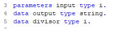
Data declaration
A typical procedural ABAP program consists of type definitions and data declarations. The data declarations describe the data structure that the program uses when it runs.
Parameters are components of a selection screen that are assigned a global elementary data object in the ABAP program and an input field on the selection screen.
So, after running our example. In a SAP GUI system or in eclipse you would have to press F8 to run a program, before you should have saved (Ctrl + s) and activated (Ctrl + F3) your program. After these three steps, you will see that parameters is a data declaration that opens an additional screen (dynpro) in the SAP GUI that receives your input variable.
ABAP has three main types of data: elementary types, complex types and reference types. In our example, only elementary types are used. Therefore, we will only give a brief overview of them in the following table:
Data Type
Description
Initial Size
Valid Size
Initial Value
C
Alphanumeric characters
1 character
1 – 65,535 characters
space
N
Digits 0-9
1 character
1 – 65,535 characters
Character zero
D
Data character YYYYMMDD
8 characters
8 characters
Character zeros
T
Time character HHMMSS
8 characters
8 characters
Character zeros
X
Hexadecimal field
1 byte
1 – 65,535 bytes
P
Packed Numbers
8 bytes
1 – 16 bytes
0
I
Integers Range 2^31-1 to 2^31
4 bytes
4 bytes
0
F
8 bytes
8 bytes
0
STRING
Like C, but has a variable length
XSTRING
Like X, but has a variable length
Overview elementary types in ABAP
DO/ENDDO and WHILE/ENDWHILE
In ABAP there are two loops that could have helped us solve our prime factor exercise: while/endwhile or do/enddo.
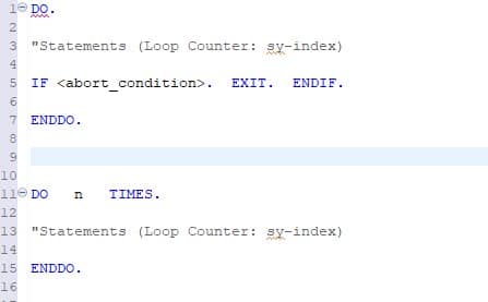
DO/ENDDO: Unconditional and indexed loops:
The block of statements between DO and ENDDO is executed continuously until the loop is exited using exit statements such as EXIT. Specify the maximum number of loop passes, otherwise you may get an infinite loop.
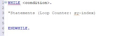
WHILE/ENDWHILE: Header-controlled loops
The statement block between WHILE and ENDWHILE is executed until the specified condition is no longer true. The condition is always checked before the statement block is executed.
WRITE
One of the very basic ABAP statements used to display data on the screen is the WRITE statement.
In our example, the backslash starts a new line for each output number.
Additional information.
For additional information, see the SAP keyword documentation:
TL;DR: In this Blogpost we will look at some data modeling methods to be used in ABAP programs. While other methods are more intuitive and easy to learn, the preferred method for experienced ABAP developers will usually be CDS Views.
Development in ABAP, a programming language used for ERP purposes, will unavoidably intersect with the task of data modeling. While the ABAP application itself contains the processing logic of the data, the modeling can be done in various ways, either within or outside the ABAP code. This article is aimed at new developers that have yet to see the many options for creating data models to be consumed by ABAP programs. It is not intended to provide a detailed explanation of each modeling method, but rather to provide a quick overview of their usage and capabilities.
Data modeling is the task of gathering data from various sources and combining and processing it into more concise data for the end user. As different data sources are often used in a similar context for different tasks, creating reusable models that can be consumed by different applications becomes a routine task. Reusable data modeling in ABAP-based programs is done using views. Like database tables, views are consumed in ABAP programs using Open SQL calls. In the following, we will be discussing the ABAP Dictionary View, the CDS View and the HANA exclusive Calculation View.
ABAP Dictionary View
The view most developers will be introduced to first is the ABAP Dictionary View. It is created with the ABAP Dictionary (SE11). It provides the option to choose several database tables (1) and collect them into a new table by choosing the desired columns (2). This is done by providing the shared columns (Join Conditions) of the underlying tables (3) and simple selection conditions (4). It does the bare minimum of data modeling; choosing which data should be displayed in a single table. The SQL equivalent of this is an inner JOIN. If your goal is to simply queue a few columns of related tables to be consumed by your ABAP code, the dictionary view is an easy way to do so.
Fig. 1: Creating an ABAP Dictionary View with the ABAP Dictionary (left) and providing data sources and conditions for the view (right).
While the ABAP Dictionary has some additional features like choosing the buffering type and inheriting field labels from its underlying data sources, any further processing of the data and supplementing technical information will have to be done in the ABAP program itself, either through lengthy SQL calls on the view or the ABAP List Viewer. The goal of data modeling is to reuse as much of the model as possible without having to code for each program individually. This makes the dictionary view the least efficient option but the easiest to understand and access since it is a simplified standard tool of the SAP GUI. It does not require any additional program or coding experience but has the fewest options.
CDS View
With the introduction of the powerful HANA databases, SAP developed views, designed for pushing computational tasks from the application layer (the ABAP program) to the database. These new views provide a lot more SQL features that not only improve performance but were also attractive for modeling purposes. But these Core Data Services (CDS) Views are not exclusive to HANA. A generic version, ABAP CDS, can be used database-independently and still provides most features of the HANA-specific CDS Views. They have a crucial role in modern SAP architecture. SAP S/4HANA uses models specifically built around CDS Views e.g., building entire Fiori Apps with the Restful ABAP Programming model. Even today, CDS is further evolving with quality-of-life improvements like CDS View Entities, a new, advanced CDS View type that provides more features and removed some redundancies of CDS Views. Creating and maintaining CDS Views is only possible with the ABAP Development Tools (ADT) accessible through Eclipse, but viewing them is still possible with the SAP GUI. They can be consumed by any ABAP program with Open SQL.
Modeling and features
So, what are these features, and what does a CDS View look like? An example can be seen in the image below. The first noticeable difference to ABAP dictionary views is: It is code-based. Every detail about the view is written down in a new line of code instead of clicking through menus and buttons. This is not limited to just the content of the view but also its technical properties. Let us start by looking at the core of a basic CDS View. You provide the source tables, the columns to be displayed, optional aliases, and a filtering condition for the data to be retrieved. One might say that it is just an SQL code. Because it is.
Fig. 2: Creating a CDS View in ADT (left). Core structure of a CDS View (right)1.
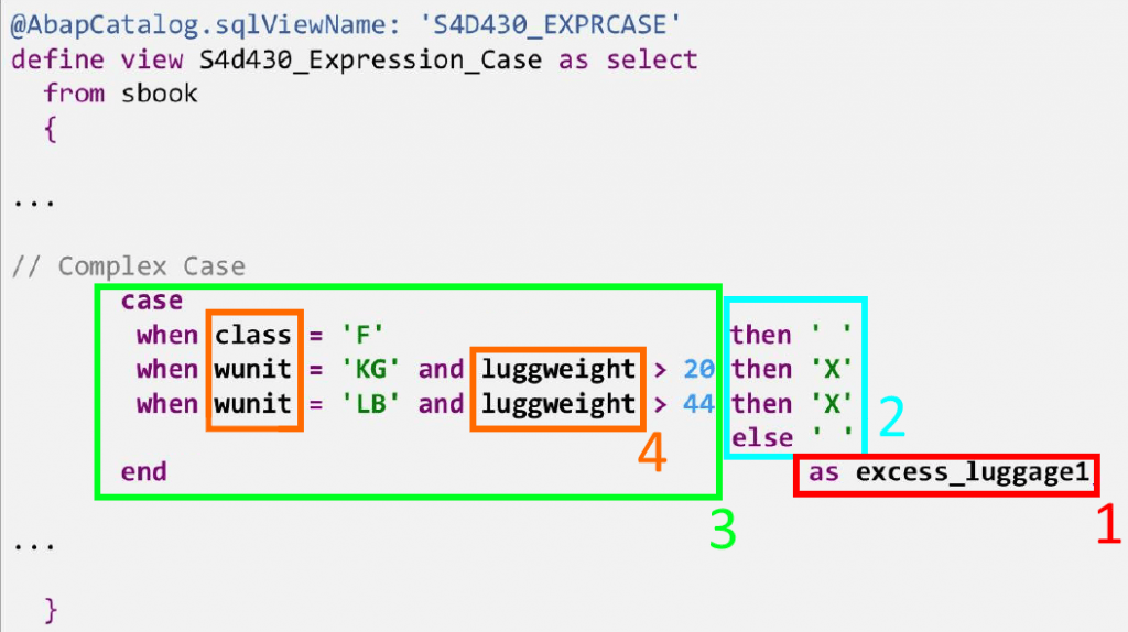
As with SQL in ABAP programs, CDS Views include features like expressions and functions. The example below shows how a CDS View defines a new column (1), whose value (2) depends on a more complex logical case expression (3) using data (4) from the underlying source tables. Arithmetic expressions (additions, divisions, etc.) and functions (rounding, modulo function, etc.), string functions (substring, word length, etc.), aggregations, and many other SQL features are, of course, also possible.
Fig. 3: Complex case expression within a CDS View
Annotations
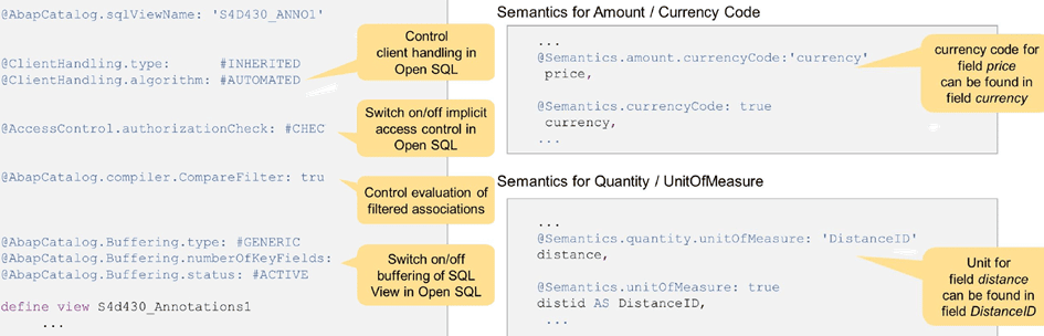
CDS features are not limited to the capabilities of SQL. The View can be enriched with semantic information using annotations. Annotations are simply expressions that define a property of the entire view or one of its elements, preceded by an “@“. Examples for both can be seen in the image below:
Setting buffering options for the view.
Specifying access control for when an ABAP program calls the view.
Defining the relationship between a column containing a value and the column containing the corresponding unit or currency.
Fig. 4: Annotations in CDS Views.1
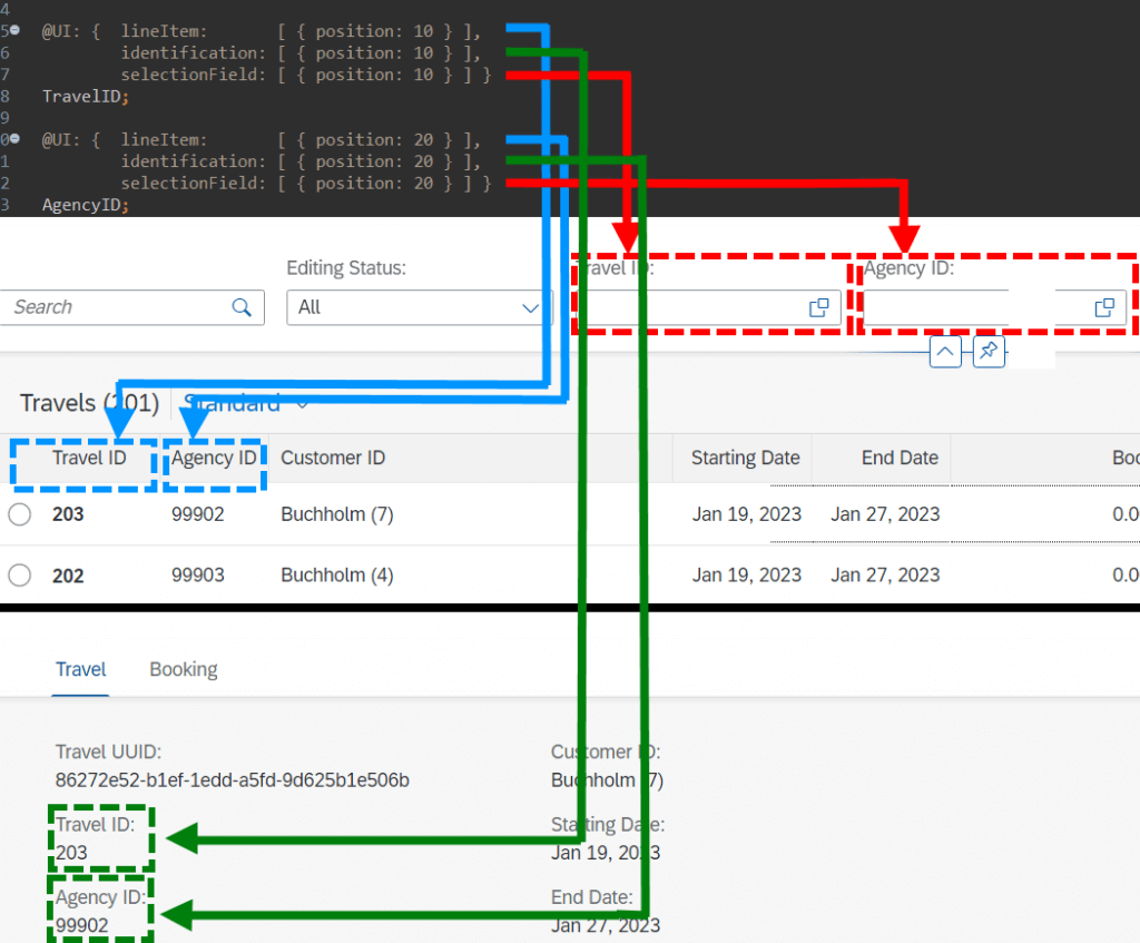
These make up only a very small fraction of all annotations. The possibilities range from general technical information to Framework-specific annotations e.g., how a User Interface should display an element of the view. They allow the Backend Developer to design entire SAP Fiori App UIs with relative ease. The image below showcases example annotations on the TravelID and AgencyID columns of the classical SAP ‘Travel Scenario’ to define some UI properties without any frontend coding:
@UI.lineItem to add the element to the list view of entries
@UI.Identification to add the element to the object page of a selected entry
@UI.SelectionField to add a search field for the element to the UI
Fig. 5: Designing UI elements in CDS with annotations.
Some additional features
Listing all the capabilities of CDS views would take too long and is not in the scope of this simple introduction. But to finish off, here are a few further interesting capabilities of CDS:
CDS Views can define input parameters that the consuming ABAP program can then provide.
They allow you to define which data should be accessible to which user roles. Before, this had to be done within the ABAP program itself (statement ‘AUTHORITY-CHECK’).
CDS Views can be enhanced. For example, a customer can create an Extention View (same structure and syntax) that adds further columns and semantic information to the view.
CDS Views can use other CDS Views as data sources. This is not possible with ABAP dictionary views.
Building views is not limited to just consuming database tables on the system. CDS Views can for example, queue data remotely through OData services.
A new, advanced type of relationship between data sources, called ‘Associations’. Compared to Joins, they can provide further information, like the cardinality between data sources. Furthermore, they act like a ‘Join on demand’, meaning the view can just show the ‘main’ data source and only joins the additional sources, if they are requested.
Calculation View
As SAP HANA completely changed the capabilities of databases, the design principles for previous programs and services became obsolete and inefficient. The goal of HANA is to push as much workload as possible away from the application layer to the database. To do this, SAP created a dedicated view called HANA Views, the most prominent one being Calculation Views. Both CDS Views and Calculation Views are designed to create the data model and all its logic on the database and send the results to the consuming program. CDS HANA Views are handled on the application layer but generate the actual model on the database, while Calculation Views are handled directly on the database and then consumed by the program. A more important difference for the developer is the modeling.
Modeling
The most glaring difference is that it is graphical. For most purposes, modeling of calculation views can be done almost exclusively without any code. Like with dictionary views, you set properties by clicking through menus, but it comes with a more intuitive graphical interface. Calculation Views can only be created, edited, and viewed in HANA Studio (deprecated) and SAP Web IDE (new versions).
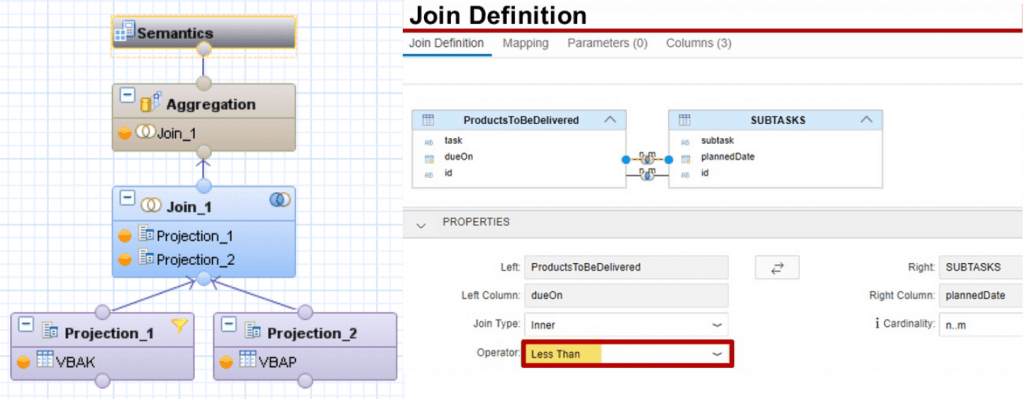
Each modeling step is done with a node. To get an overview of the modeling, let us look at the image below, which shows a simple case of joining two data sources. The first layer consists of two Projection nodes. Each of them selects columns from one data source to be projected to the next layer. On the second layer, a Join node combines the data sources. By navigating to the Join menu, the Join Condition and additional details like cardinality and Join type are set. On the next layer, the data is aggregated; only the sum, maximum, minimum, etc. of grouped entries is displayed by carefully defining the aggregation order and conditions. At the top level is always the Semantic node that is used to define the behaviour and meaning of each column of the final view to be consumed. Similar to annotations of CDS Views, the Semantic node can be used to provide a large variety of technical information to individual columns, like currency codes, labels, data types, data masking, and many more.
Fig. 6: Layers for the creation of a calculation view (left)2 and Join Definition for a Join node (right)3. Images unrelated to each other.
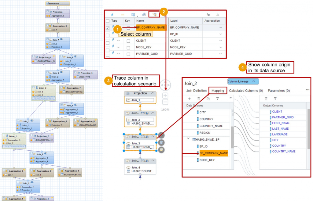
While modeling Calculation Views can take some time to learn simply due to their many features, an advantage over CDS Views is that they require no coding experience. Learning it can be more intuitive, making it especially attractive for data modelers who are not necessarily ABAP developers. Another possible advantage of calculation views can be considered by looking at the image below. Convoluted models with many Join and processing steps could be confusing to work with. Having the entire model displayed in one diagram could be easier to follow than an equivalent script-based model. To further simplify this, calculation views allow the modeler to follow a column at higher node levels to track back to its origin.
Example of a more complex Calculation View (left) 4. Showing the Lineage of a view (right).3 Images unrelated to each other.
Some last points
The features provided by Calculation Views are numerous. Like with CDS Views, entire books are written about their capabilities. This article is merely a short overview but some further noteworthy points regarding Calculation Views:
Like with CDS Views, parameters can be defined.
Calculation Views can use other Calculation Views.
You can provide access control at the database level through so-called Analytic Privileges.
More complex features, that are not covered in the graphical model, can be supplemented with Functions andProcedures, reusable blocks of SQLScript code, that can be consumed in any Calculation View and even be used directly in ABAP programs using special methods called ABAP managed Database Procedures (recommended) or by creating a proxy object for the procedure (outdated).
HANA Views fully utilize the capabilities of SAP HANA. They are designed to get the best performance out of its in-memory technology but also have full access to the integrated Application Function Libraries, a series of C++ procedures designed to handle complex computations with great performance. Note that the usage of each library (Business Function Library, Predictive Analysis Library, Automated Predictive Library, Extended Machine Learning Library) requires its own license.
During the early phases of HANA Views, Analytic Views and Attribute Views were used to handle the measures (quantities) and the corresponding dimensions (elements describing the measures like customers, products etc.), respectively. These were later integrated into Calculation Views and are now obsolete. Also deprecated is the fully scripted Calculation View.
A disadvantage of Calculation Views is that they cannot be used with Open SQL. For an ABAP program to consume them, it will require an intermediate step. Some of those are:
A Native SQL interface like ABAP Database Connectivity (ADBC) must be called within the program.
Creating a Proxy Object for the view, an External View, which can be consumed with Open SQL.
Consume the Calculation View in a CDS View using a CDS Table Function, then consume the CDS View in the ABAP program.
While Calculation Views can be used by ABAP programs, they are not managed by ABAP and thus require a separate lifecycle.
Summary
Let us summarize the advantages and disadvantages of each option:
ABAP Dictionary Views are easy to understand and available as a standard tool in the SAP GUI, but provide very few options. Further modeling requirements will unavoidably have to be done in the ABAP program. Good for beginners who only want simple Joins.
CDS Views have far more features that not only provide more capabilities but are also more comfortable to use once one is used to them. They are perfectly usable with ABAP but require ADT and knowledge of SQL-sublanguages (DDL, DCL and DML) to code them properly. Good for experienced data modelers that want to use the full scope of modeling features in ABAP programs.
Calculation Views are a code-free alternative to CDS Views regarding its features, but they can be only used with HANA databases. It requires the use of the SAP Web IDE, and consumption in ABAP code needs an intermediate step. Good for data modelers who are not experienced in ABAP and CDS or simply prefer graphical over scripted modeling.
Development in ABAP, a programming language used for ERP purposes, will unavoidably intersect with the task of data modeling. While the ABAP application itself contains the processing logic of the data, the modeling can be done in various ways, either within or outside the ABAP code. This article is aimed at new developers that have yet to see the many options for creating data models to be consumed by ABAP programs. It is not intended to provide a detailed explanation of each modeling method, but rather to provide a quick overview of their usage and capabilities.
Data modeling is the task of gathering data from various sources and combining and processing it into more concise data for the end user. As different data sources are often used in a similar context for different tasks, creating reusable models that can be consumed by different applications becomes a routine task. Reusable data modeling in ABAP-based programs is done using views. Like database tables, views are consumed in ABAP programs using Open SQL calls. In the following, we will be discussing the ABAP Dictionary View, the CDS View and the HANA exclusive Calculation View.
ABAP Dictionary View
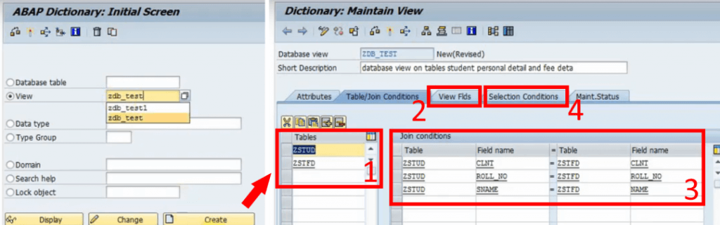
The view most developers will be introduced to first is the ABAP Dictionary View. It is created with the ABAP Dictionary (SE11). It provides the option to choose several database tables (1) and collect them into a new table by choosing the desired columns (2). This is done by providing the shared columns (Join Conditions) of the underlying tables (3) and simple selection conditions (4). It does the bare minimum of data modeling; choosing which data should be displayed in a single table. The SQL equivalent of this is an inner JOIN. If your goal is to simply queue a few columns of related tables to be consumed by your ABAP code, the dictionary view is an easy way to do so.
Fig. 1: Creating an ABAP Dictionary View with the ABAP Dictionary (left) and providing data sources and conditions for the view (right).
While the ABAP Dictionary has some additional features like choosing the buffering type and inheriting field labels from its underlying data sources, any further processing of the data and supplementing technical information will have to be done in the ABAP program itself, either through lengthy SQL calls on the view or the ABAP List Viewer. The goal of data modeling is to reuse as much of the model as possible without having to code for each program individually. This makes the dictionary view the least efficient option but the easiest to understand and access since it is a simplified standard tool of the SAP GUI. It does not require any additional program or coding experience but has the fewest options.
CDS View
With the introduction of the powerful HANA databases, SAP developed views, designed for pushing computational tasks from the application layer (the ABAP program) to the database. These new views provide a lot more SQL features that not only improve performance but were also attractive for modeling purposes. But these Core Data Services (CDS) Views are not exclusive to HANA. A generic version, ABAP CDS, can be used database-independently and still provides most features of the HANA-specific CDS Views. They have a crucial role in modern SAP architecture. SAP S/4HANA uses models specifically built around CDS Views e.g., building entire Fiori Apps with the Restful ABAP Programming model. Even today, CDS is further evolving with quality-of-life improvements like CDS View Entities, a new, advanced CDS View type that provides more features and removed some redundancies of CDS Views. Creating and maintaining CDS Views is only possible with the ABAP Development Tools (ADT) accessible through Eclipse, but viewing them is still possible with the SAP GUI. They can be consumed by any ABAP program with Open SQL.
Modeling and features
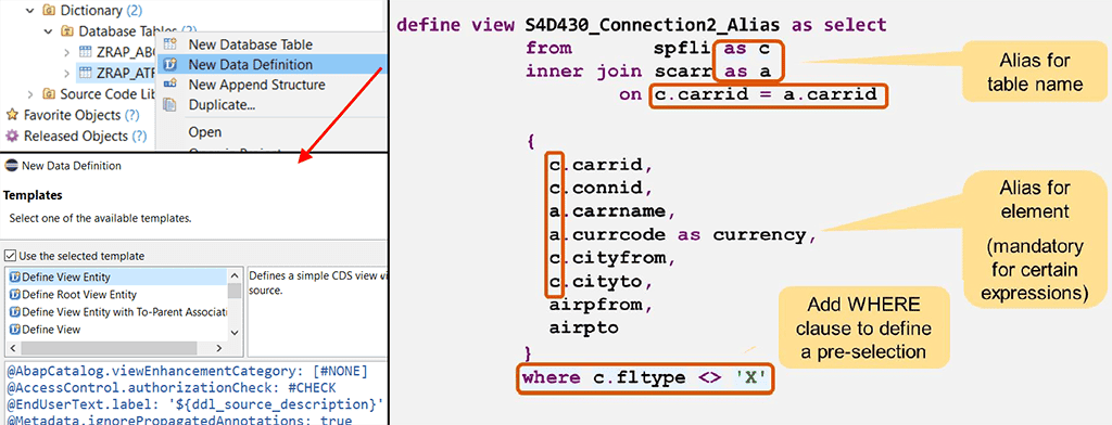
So, what are these features, and what does a CDS View look like? An example can be seen in the image below. The first noticeable difference to ABAP dictionary views is: It is code-based. Every detail about the view is written down in a new line of code instead of clicking through menus and buttons. This is not limited to just the content of the view but also its technical properties. Let us start by looking at the core of a basic CDS View. You provide the source tables, the columns to be displayed, optional aliases, and a filtering condition for the data to be retrieved. One might say that it is just an SQL code. Because it is.
Fig. 2: Creating a CDS View in ADT (left). Core structure of a CDS View (right)1.
As with SQL in ABAP programs, CDS Views include features like expressions and functions. The example below shows how a CDS View defines a new column (1), whose value (2) depends on a more complex logical case expression (3) using data (4) from the underlying source tables. Arithmetic expressions (additions, divisions, etc.) and functions (rounding, modulo function, etc.), string functions (substring, word length, etc.), aggregations, and many other SQL features are, of course, also possible.
Fig. 3: Complex case expression within a CDS View
Annotations
CDS features are not limited to the capabilities of SQL. The View can be enriched with semantic information using annotations. Annotations are simply expressions that define a property of the entire view or one of its elements, preceded by an “@“. Examples for both can be seen in the image below:
Setting buffering options for the view.
Specifying access control for when an ABAP program calls the view.
Defining the relationship between a column containing a value and the column containing the corresponding unit or currency.
Fig. 4: Annotations in CDS Views.1
These make up only a very small fraction of all annotations. The possibilities range from general technical information to Framework-specific annotations e.g., how a User Interface should display an element of the view. They allow the Backend Developer to design entire SAP Fiori App UIs with relative ease. The image below showcases example annotations on the TravelID and AgencyID columns of the classical SAP ‘Travel Scenario’ to define some UI properties without any frontend coding:
@UI.lineItem to add the element to the list view of entries
@UI.Identification to add the element to the object page of a selected entry
@UI.SelectionField to add a search field for the element to the UI
Fig. 5: Designing UI elements in CDS with annotations.
Some additional features
Listing all the capabilities of CDS views would take too long and is not in the scope of this simple introduction. But to finish off, here are a few further interesting capabilities of CDS:
CDS Views can define input parameters that the consuming ABAP program can then provide.
They allow you to define which data should be accessible to which user roles. Before, this had to be done within the ABAP program itself (statement ‘AUTHORITY-CHECK’).
CDS Views can be enhanced. For example, a customer can create an Extention View (same structure and syntax) that adds further columns and semantic information to the view.
CDS Views can use other CDS Views as data sources. This is not possible with ABAP dictionary views.
Building views is not limited to just consuming database tables on the system. CDS Views can for example, queue data remotely through OData services.
A new, advanced type of relationship between data sources, called ‘Associations’. Compared to Joins, they can provide further information, like the cardinality between data sources. Furthermore, they act like a ‘Join on demand’, meaning the view can just show the ‘main’ data source and only joins the additional sources, if they are requested.
Calculation View
As SAP HANA completely changed the capabilities of databases, the design principles for previous programs and services became obsolete and inefficient. The goal of HANA is to push as much workload as possible away from the application layer to the database. To do this, SAP created a dedicated view called HANA Views, the most prominent one being Calculation Views. Both CDS Views and Calculation Views are designed to create the data model and all its logic on the database and send the results to the consuming program. CDS HANA Views are handled on the application layer but generate the actual model on the database, while Calculation Views are handled directly on the database and then consumed by the program. A more important difference for the developer is the modeling.
Modeling
The most glaring difference is that it is graphical. For most purposes, modeling of calculation views can be done almost exclusively without any code. Like with dictionary views, you set properties by clicking through menus, but it comes with a more intuitive graphical interface. Calculation Views can only be created, edited, and viewed in HANA Studio (deprecated) and SAP Web IDE (new versions).
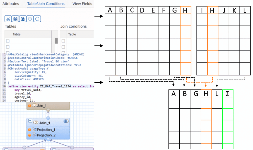
Each modeling step is done with a node. To get an overview of the modeling, let us look at the image below, which shows a simple case of joining two data sources. The first layer consists of two Projection nodes. Each of them selects columns from one data source to be projected to the next layer. On the second layer, a Join node combines the data sources. By navigating to the Join menu, the Join Condition and additional details like cardinality and Join type are set. On the next layer, the data is aggregated; only the sum, maximum, minimum, etc. of grouped entries is displayed by carefully defining the aggregation order and conditions. At the top level is always the Semantic node that is used to define the behaviour and meaning of each column of the final view to be consumed. Similar to annotations of CDS Views, the Semantic node can be used to provide a large variety of technical information to individual columns, like currency codes, labels, data types, data masking, and many more.
Fig. 6: Layers for the creation of a calculation view (left)2 and Join Definition for a Join node (right)3. Images unrelated to each other.
While modeling Calculation Views can take some time to learn simply due to their many features, an advantage over CDS Views is that they require no coding experience. Learning it can be more intuitive, making it especially attractive for data modelers who are not necessarily ABAP developers. Another possible advantage of calculation views can be considered by looking at the image below. Convoluted models with many Join and processing steps could be confusing to work with. Having the entire model displayed in one diagram could be easier to follow than an equivalent script-based model. To further simplify this, calculation views allow the modeler to follow a column at higher node levels to track back to its origin.
Example of a more complex Calculation View (left) 4. Showing the Lineage of a view (right).3 Images unrelated to each other.
Some last points
The features provided by Calculation Views are numerous. Like with CDS Views, entire books are written about their capabilities. This article is merely a short overview but some further noteworthy points regarding Calculation Views:
Like with CDS Views, parameters can be defined.
Calculation Views can use other Calculation Views.
You can provide access control at the database level through so-called Analytic Privileges.
More complex features, that are not covered in the graphical model, can be supplemented with Functions andProcedures, reusable blocks of SQLScript code, that can be consumed in any Calculation View and even be used directly in ABAP programs using special methods called ABAP managed Database Procedures (recommended) or by creating a proxy object for the procedure (outdated).
HANA Views fully utilize the capabilities of SAP HANA. They are designed to get the best performance out of its in-memory technology but also have full access to the integrated Application Function Libraries, a series of C++ procedures designed to handle complex computations with great performance. Note that the usage of each library (Business Function Library, Predictive Analysis Library, Automated Predictive Library, Extended Machine Learning Library) requires its own license.
During the early phases of HANA Views, Analytic Views and Attribute Views were used to handle the measures (quantities) and the corresponding dimensions (elements describing the measures like customers, products etc.), respectively. These were later integrated into Calculation Views and are now obsolete. Also deprecated is the fully scripted Calculation View.
A disadvantage of Calculation Views is that they cannot be used with Open SQL. For an ABAP program to consume them, it will require an intermediate step. Some of those are:
A Native SQL interface like ABAP Database Connectivity (ADBC) must be called within the program.
Creating a Proxy Object for the view, an External View, which can be consumed with Open SQL.
Consume the Calculation View in a CDS View using a CDS Table Function, then consume the CDS View in the ABAP program.
While Calculation Views can be used by ABAP programs, they are not managed by ABAP and thus require a separate lifecycle.
Summary
Let us summarize the advantages and disadvantages of each option:
ABAP Dictionary Views are easy to understand and available as a standard tool in the SAP GUI, but provide very few options. Further modeling requirements will unavoidably have to be done in the ABAP program. Good for beginners who only want simple Joins.
CDS Views have far more features that not only provide more capabilities but are also more comfortable to use once one is used to them. They are perfectly usable with ABAP but require ADT and knowledge of SQL-sublanguages (DDL, DCL and DML) to code them properly. Good for experienced data modelers that want to use the full scope of modeling features in ABAP programs.
Calculation Views are a code-free alternative to CDS Views regarding its features, but they can be only used with HANA databases. It requires the use of the SAP Web IDE, and consumption in ABAP code needs an intermediate step. Good for data modelers who are not experienced in ABAP and CDS or simply prefer graphical over scripted modeling.